1. Raster Data#
In scikit-map, the class RasterData is responsible to implement reading, processing and writing operations. To understand how it works let’s load the NDVI toy dataset provided by default.
[1]:
import warnings
warnings.filterwarnings("ignore")
from skmap.data import toy
rdata = toy.ndvi_rdata(gappy=True)
[08:17:34] RasterData with 24 rasters (band: 1) and 1 group(s)
[08:17:34] Reading 24 raster file(s) using 4 workers
[08:17:35] Read array shape: (256, 256, 24)
A RasterData instance is basically a Pandas DataFrame accessible through the info attribute
[2]:
rdata.info
[2]:
| group | input_path | input_band | start_date | end_date | temporal | name | |
|---|---|---|---|---|---|---|---|
| 0 | ndvi | /home/opengeohub/src/scikit-map/skmap/data/toy... | 1 | 2014-12-02 | 2015-03-20 | True | ndvi_landsat.ard1_p50_30m_s_20141202_20150320_... |
| 1 | ndvi | /home/opengeohub/src/scikit-map/skmap/data/toy... | 1 | 2015-03-21 | 2015-06-24 | True | ndvi_landsat.ard1_p50_30m_s_20150321_20150624_... |
| 2 | ndvi | /home/opengeohub/src/scikit-map/skmap/data/toy... | 1 | 2015-06-25 | 2015-09-12 | True | ndvi_landsat.ard1_p50_30m_s_20150625_20150912_... |
| 3 | ndvi | /home/opengeohub/src/scikit-map/skmap/data/toy... | 1 | 2015-09-13 | 2015-12-01 | True | ndvi_landsat.ard1_p50_30m_s_20150913_20151201_... |
| 4 | ndvi | /home/opengeohub/src/scikit-map/skmap/data/toy... | 1 | 2015-12-02 | 2016-03-20 | True | ndvi_landsat.ard1_p50_30m_s_20151202_20160320_... |
| 5 | ndvi | /home/opengeohub/src/scikit-map/skmap/data/toy... | 1 | 2016-03-21 | 2016-06-24 | True | ndvi_landsat.ard1_p50_30m_s_20160321_20160624_... |
| 6 | ndvi | /home/opengeohub/src/scikit-map/skmap/data/toy... | 1 | 2016-06-25 | 2016-09-12 | True | ndvi_landsat.ard1_p50_30m_s_20160625_20160912_... |
| 7 | ndvi | /home/opengeohub/src/scikit-map/skmap/data/toy... | 1 | 2016-09-13 | 2016-12-01 | True | ndvi_landsat.ard1_p50_30m_s_20160913_20161201_... |
| 8 | ndvi | /home/opengeohub/src/scikit-map/skmap/data/toy... | 1 | 2016-12-02 | 2017-03-20 | True | ndvi_landsat.ard1_p50_30m_s_20161202_20170320_... |
| 9 | ndvi | /home/opengeohub/src/scikit-map/skmap/data/toy... | 1 | 2017-03-21 | 2017-06-24 | True | ndvi_landsat.ard1_p50_30m_s_20170321_20170624_... |
| 10 | ndvi | /home/opengeohub/src/scikit-map/skmap/data/toy... | 1 | 2017-06-25 | 2017-09-12 | True | ndvi_landsat.ard1_p50_30m_s_20170625_20170912_... |
| 11 | ndvi | /home/opengeohub/src/scikit-map/skmap/data/toy... | 1 | 2017-09-13 | 2017-12-01 | True | ndvi_landsat.ard1_p50_30m_s_20170913_20171201_... |
| 12 | ndvi | /home/opengeohub/src/scikit-map/skmap/data/toy... | 1 | 2017-12-02 | 2018-03-20 | True | ndvi_landsat.ard1_p50_30m_s_20171202_20180320_... |
| 13 | ndvi | /home/opengeohub/src/scikit-map/skmap/data/toy... | 1 | 2018-03-21 | 2018-06-24 | True | ndvi_landsat.ard1_p50_30m_s_20180321_20180624_... |
| 14 | ndvi | /home/opengeohub/src/scikit-map/skmap/data/toy... | 1 | 2018-06-25 | 2018-09-12 | True | ndvi_landsat.ard1_p50_30m_s_20180625_20180912_... |
| 15 | ndvi | /home/opengeohub/src/scikit-map/skmap/data/toy... | 1 | 2018-09-13 | 2018-12-01 | True | ndvi_landsat.ard1_p50_30m_s_20180913_20181201_... |
| 16 | ndvi | /home/opengeohub/src/scikit-map/skmap/data/toy... | 1 | 2018-12-02 | 2019-03-20 | True | ndvi_landsat.ard1_p50_30m_s_20181202_20190320_... |
| 17 | ndvi | /home/opengeohub/src/scikit-map/skmap/data/toy... | 1 | 2019-03-21 | 2019-06-24 | True | ndvi_landsat.ard1_p50_30m_s_20190321_20190624_... |
| 18 | ndvi | /home/opengeohub/src/scikit-map/skmap/data/toy... | 1 | 2019-06-25 | 2019-09-12 | True | ndvi_landsat.ard1_p50_30m_s_20190625_20190912_... |
| 19 | ndvi | /home/opengeohub/src/scikit-map/skmap/data/toy... | 1 | 2019-09-13 | 2019-12-01 | True | ndvi_landsat.ard1_p50_30m_s_20190913_20191201_... |
| 20 | ndvi | /home/opengeohub/src/scikit-map/skmap/data/toy... | 1 | 2019-12-02 | 2020-03-20 | True | ndvi_landsat.ard1_p50_30m_s_20191202_20200320_... |
| 21 | ndvi | /home/opengeohub/src/scikit-map/skmap/data/toy... | 1 | 2020-03-21 | 2020-06-24 | True | ndvi_landsat.ard1_p50_30m_s_20200321_20200624_... |
| 22 | ndvi | /home/opengeohub/src/scikit-map/skmap/data/toy... | 1 | 2020-06-25 | 2020-09-12 | True | ndvi_landsat.ard1_p50_30m_s_20200625_20200912_... |
| 23 | ndvi | /home/opengeohub/src/scikit-map/skmap/data/toy... | 1 | 2020-09-13 | 2020-12-01 | True | ndvi_landsat.ard1_p50_30m_s_20200913_20201201_... |
…and a 3D Nunmpy array, the array attribute with x, y and time as dimensions.
[3]:
rdata.array.shape
[3]:
(256, 256, 24)
The array can be filtered and subset using info.
[4]:
rdata.array[:, :, (rdata.info["end_date"] >= "2020-01-01")].shape
[4]:
(256, 256, 4)
However you can use the filter method passing a query expression as parameter.
[5]:
rdata.filter('start_date > "2020-01-01"', return_array=True).shape
[5]:
(256, 256, 3)
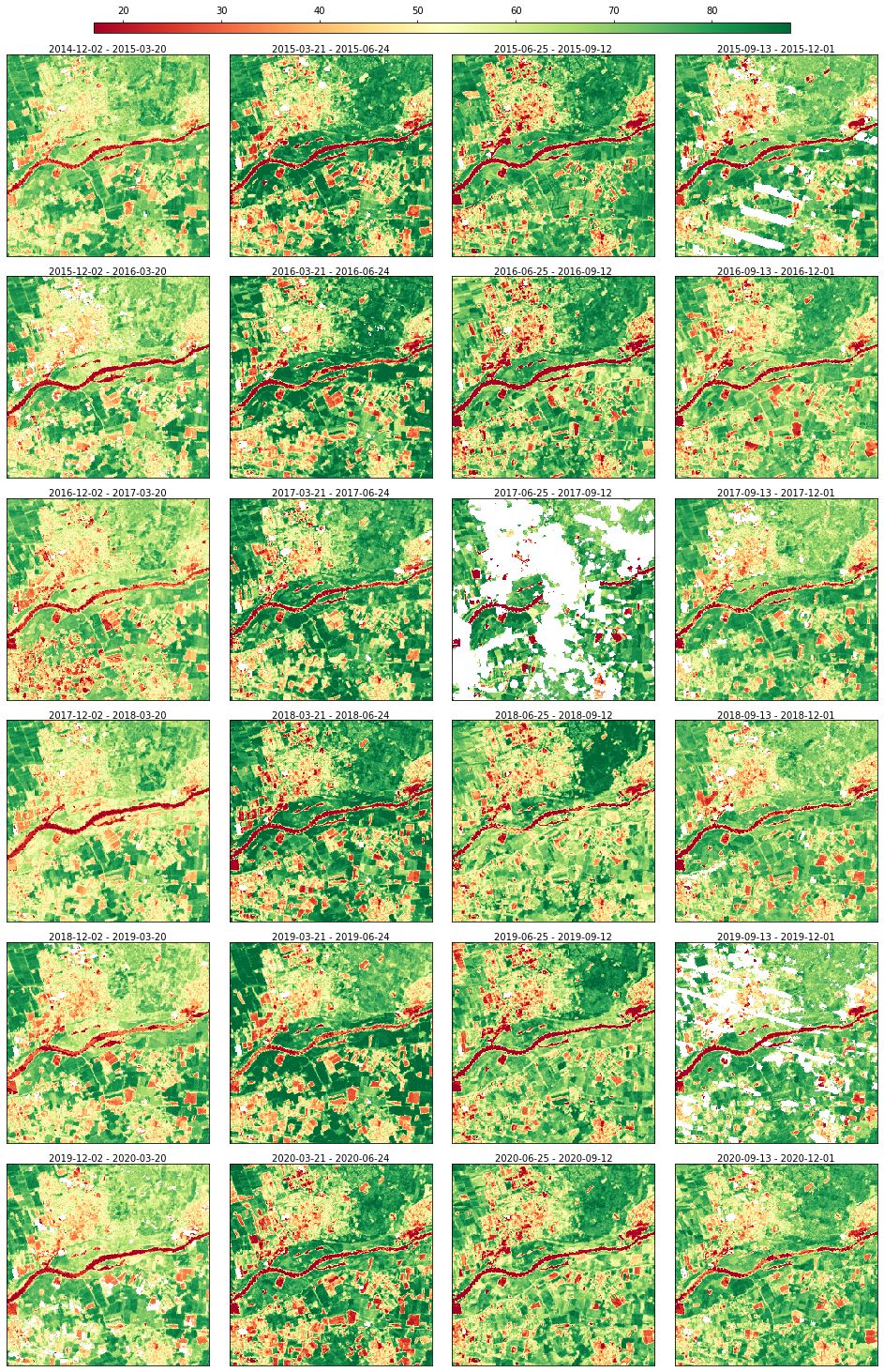
The data can be visualized through a static plot
[6]:
rdata.plot(cmap="RdYlGn", img_title_text="date")
[6]:
… and an animation.
[ ]:
rdata.animate(cmap="RdYlGn", img_title_text="date")
After visualizing the data, it’s possible to notice some data gaps in the NDVI series.
Scikit-map supports several data processing task including gapfilling, smoothing, time aggregation, math operations, trend analysis, etc. Let’s run a gapfilling process and visualize the result.
[9]:
from skmap.io import process
rdata = rdata.run(process.SeasConvFill(season_size=4), drop_input=True)
rdata.animate(cmap="RdYlGn", img_title_text="date")
[08:18:06] Running SeasConvFill on (256, 256, 24) for ndvi.seasconv group
[08:18:06] Dropping data and info for ndvi.seasconv group
[08:18:06] Execution time for SeasConvFill: 0.48 segs
[9]:
The info attribute shows that the new group ndvi.seasconv was created, and the old one ndvi was deleted according to drop_input=True.
[10]:
rdata.info
[10]:
| group | input_path | input_band | start_date | end_date | temporal | name | |
|---|---|---|---|---|---|---|---|
| 0 | ndvi.seasconv.seasconv | /home/opengeohub/src/scikit-map/skmap/data/toy... | 1 | 2014-12-02 | 2015-03-20 | True | skmap_seasconv_ndvi.seasconv_20141202_20150320 |
| 1 | ndvi.seasconv.seasconv | /home/opengeohub/src/scikit-map/skmap/data/toy... | 1 | 2015-03-21 | 2015-06-24 | True | skmap_seasconv_ndvi.seasconv_20150321_20150624 |
| 2 | ndvi.seasconv.seasconv | /home/opengeohub/src/scikit-map/skmap/data/toy... | 1 | 2015-06-25 | 2015-09-12 | True | skmap_seasconv_ndvi.seasconv_20150625_20150912 |
| 3 | ndvi.seasconv.seasconv | /home/opengeohub/src/scikit-map/skmap/data/toy... | 1 | 2015-09-13 | 2015-12-01 | True | skmap_seasconv_ndvi.seasconv_20150913_20151201 |
| 4 | ndvi.seasconv.seasconv | /home/opengeohub/src/scikit-map/skmap/data/toy... | 1 | 2015-12-02 | 2016-03-20 | True | skmap_seasconv_ndvi.seasconv_20151202_20160320 |
| 5 | ndvi.seasconv.seasconv | /home/opengeohub/src/scikit-map/skmap/data/toy... | 1 | 2016-03-21 | 2016-06-24 | True | skmap_seasconv_ndvi.seasconv_20160321_20160624 |
| 6 | ndvi.seasconv.seasconv | /home/opengeohub/src/scikit-map/skmap/data/toy... | 1 | 2016-06-25 | 2016-09-12 | True | skmap_seasconv_ndvi.seasconv_20160625_20160912 |
| 7 | ndvi.seasconv.seasconv | /home/opengeohub/src/scikit-map/skmap/data/toy... | 1 | 2016-09-13 | 2016-12-01 | True | skmap_seasconv_ndvi.seasconv_20160913_20161201 |
| 8 | ndvi.seasconv.seasconv | /home/opengeohub/src/scikit-map/skmap/data/toy... | 1 | 2016-12-02 | 2017-03-20 | True | skmap_seasconv_ndvi.seasconv_20161202_20170320 |
| 9 | ndvi.seasconv.seasconv | /home/opengeohub/src/scikit-map/skmap/data/toy... | 1 | 2017-03-21 | 2017-06-24 | True | skmap_seasconv_ndvi.seasconv_20170321_20170624 |
| 10 | ndvi.seasconv.seasconv | /home/opengeohub/src/scikit-map/skmap/data/toy... | 1 | 2017-06-25 | 2017-09-12 | True | skmap_seasconv_ndvi.seasconv_20170625_20170912 |
| 11 | ndvi.seasconv.seasconv | /home/opengeohub/src/scikit-map/skmap/data/toy... | 1 | 2017-09-13 | 2017-12-01 | True | skmap_seasconv_ndvi.seasconv_20170913_20171201 |
| 12 | ndvi.seasconv.seasconv | /home/opengeohub/src/scikit-map/skmap/data/toy... | 1 | 2017-12-02 | 2018-03-20 | True | skmap_seasconv_ndvi.seasconv_20171202_20180320 |
| 13 | ndvi.seasconv.seasconv | /home/opengeohub/src/scikit-map/skmap/data/toy... | 1 | 2018-03-21 | 2018-06-24 | True | skmap_seasconv_ndvi.seasconv_20180321_20180624 |
| 14 | ndvi.seasconv.seasconv | /home/opengeohub/src/scikit-map/skmap/data/toy... | 1 | 2018-06-25 | 2018-09-12 | True | skmap_seasconv_ndvi.seasconv_20180625_20180912 |
| 15 | ndvi.seasconv.seasconv | /home/opengeohub/src/scikit-map/skmap/data/toy... | 1 | 2018-09-13 | 2018-12-01 | True | skmap_seasconv_ndvi.seasconv_20180913_20181201 |
| 16 | ndvi.seasconv.seasconv | /home/opengeohub/src/scikit-map/skmap/data/toy... | 1 | 2018-12-02 | 2019-03-20 | True | skmap_seasconv_ndvi.seasconv_20181202_20190320 |
| 17 | ndvi.seasconv.seasconv | /home/opengeohub/src/scikit-map/skmap/data/toy... | 1 | 2019-03-21 | 2019-06-24 | True | skmap_seasconv_ndvi.seasconv_20190321_20190624 |
| 18 | ndvi.seasconv.seasconv | /home/opengeohub/src/scikit-map/skmap/data/toy... | 1 | 2019-06-25 | 2019-09-12 | True | skmap_seasconv_ndvi.seasconv_20190625_20190912 |
| 19 | ndvi.seasconv.seasconv | /home/opengeohub/src/scikit-map/skmap/data/toy... | 1 | 2019-09-13 | 2019-12-01 | True | skmap_seasconv_ndvi.seasconv_20190913_20191201 |
| 20 | ndvi.seasconv.seasconv | /home/opengeohub/src/scikit-map/skmap/data/toy... | 1 | 2019-12-02 | 2020-03-20 | True | skmap_seasconv_ndvi.seasconv_20191202_20200320 |
| 21 | ndvi.seasconv.seasconv | /home/opengeohub/src/scikit-map/skmap/data/toy... | 1 | 2020-03-21 | 2020-06-24 | True | skmap_seasconv_ndvi.seasconv_20200321_20200624 |
| 22 | ndvi.seasconv.seasconv | /home/opengeohub/src/scikit-map/skmap/data/toy... | 1 | 2020-06-25 | 2020-09-12 | True | skmap_seasconv_ndvi.seasconv_20200625_20200912 |
| 23 | ndvi.seasconv.seasconv | /home/opengeohub/src/scikit-map/skmap/data/toy... | 1 | 2020-09-13 | 2020-12-01 | True | skmap_seasconv_ndvi.seasconv_20200913_20201201 |
RasterData supports the execution of multiple processing tasks through fluent interface relying extensively on method chaining.
Let’s testing it by
Loading again the gappy NDVI time-series,
Running the gapfilling approach, and
aggregating the gapffiled data by year using two time reducers operations (standard deviation and percentile 50th).
[11]:
rdata = (
toy.ndvi_rdata(
gappy=True
# Gapfilling time-series by seasonal convolution
)
.run(
process.SeasConvFill(season_size=4),
drop_input=True,
# Renaming back the output to ndvi
)
.rename(
groups={"ndvi.seasconv": "ndvi"}
# Running yearly aggregation by std. and percentile 50th
)
.run(
process.TimeAggregate(
time=[process.TimeEnum.YEARLY], operations=["p50", "std"]
),
group=["ndvi"],
)
)
rdata.info
[08:18:13] RasterData with 24 rasters (band: 1) and 1 group(s)
[08:18:13] Reading 24 raster file(s) using 4 workers
[08:18:14] Read array shape: (256, 256, 24)
[08:18:14] Running SeasConvFill on (256, 256, 24) for ndvi group
[08:18:14] Dropping data and info for ndvi group
[08:18:14] Execution time for SeasConvFill: 0.61 segs
[08:18:14] Running TimeAggregate on (256, 256, 24) for ndvi group
[08:18:15] Execution time for TimeAggregate: 0.19 segs
[11]:
| group | input_path | input_band | start_date | end_date | temporal | name | |
|---|---|---|---|---|---|---|---|
| 0 | ndvi | /home/opengeohub/src/scikit-map/skmap/data/toy... | 1 | 2014-12-02 | 2015-03-20 | True | skmap_seasconv_ndvi_20141202_20150320 |
| 1 | ndvi | /home/opengeohub/src/scikit-map/skmap/data/toy... | 1 | 2015-03-21 | 2015-06-24 | True | skmap_seasconv_ndvi_20150321_20150624 |
| 2 | ndvi | /home/opengeohub/src/scikit-map/skmap/data/toy... | 1 | 2015-06-25 | 2015-09-12 | True | skmap_seasconv_ndvi_20150625_20150912 |
| 3 | ndvi | /home/opengeohub/src/scikit-map/skmap/data/toy... | 1 | 2015-09-13 | 2015-12-01 | True | skmap_seasconv_ndvi_20150913_20151201 |
| 4 | ndvi | /home/opengeohub/src/scikit-map/skmap/data/toy... | 1 | 2015-12-02 | 2016-03-20 | True | skmap_seasconv_ndvi_20151202_20160320 |
| 5 | ndvi | /home/opengeohub/src/scikit-map/skmap/data/toy... | 1 | 2016-03-21 | 2016-06-24 | True | skmap_seasconv_ndvi_20160321_20160624 |
| 6 | ndvi | /home/opengeohub/src/scikit-map/skmap/data/toy... | 1 | 2016-06-25 | 2016-09-12 | True | skmap_seasconv_ndvi_20160625_20160912 |
| 7 | ndvi | /home/opengeohub/src/scikit-map/skmap/data/toy... | 1 | 2016-09-13 | 2016-12-01 | True | skmap_seasconv_ndvi_20160913_20161201 |
| 8 | ndvi | /home/opengeohub/src/scikit-map/skmap/data/toy... | 1 | 2016-12-02 | 2017-03-20 | True | skmap_seasconv_ndvi_20161202_20170320 |
| 9 | ndvi | /home/opengeohub/src/scikit-map/skmap/data/toy... | 1 | 2017-03-21 | 2017-06-24 | True | skmap_seasconv_ndvi_20170321_20170624 |
| 10 | ndvi | /home/opengeohub/src/scikit-map/skmap/data/toy... | 1 | 2017-06-25 | 2017-09-12 | True | skmap_seasconv_ndvi_20170625_20170912 |
| 11 | ndvi | /home/opengeohub/src/scikit-map/skmap/data/toy... | 1 | 2017-09-13 | 2017-12-01 | True | skmap_seasconv_ndvi_20170913_20171201 |
| 12 | ndvi | /home/opengeohub/src/scikit-map/skmap/data/toy... | 1 | 2017-12-02 | 2018-03-20 | True | skmap_seasconv_ndvi_20171202_20180320 |
| 13 | ndvi | /home/opengeohub/src/scikit-map/skmap/data/toy... | 1 | 2018-03-21 | 2018-06-24 | True | skmap_seasconv_ndvi_20180321_20180624 |
| 14 | ndvi | /home/opengeohub/src/scikit-map/skmap/data/toy... | 1 | 2018-06-25 | 2018-09-12 | True | skmap_seasconv_ndvi_20180625_20180912 |
| 15 | ndvi | /home/opengeohub/src/scikit-map/skmap/data/toy... | 1 | 2018-09-13 | 2018-12-01 | True | skmap_seasconv_ndvi_20180913_20181201 |
| 16 | ndvi | /home/opengeohub/src/scikit-map/skmap/data/toy... | 1 | 2018-12-02 | 2019-03-20 | True | skmap_seasconv_ndvi_20181202_20190320 |
| 17 | ndvi | /home/opengeohub/src/scikit-map/skmap/data/toy... | 1 | 2019-03-21 | 2019-06-24 | True | skmap_seasconv_ndvi_20190321_20190624 |
| 18 | ndvi | /home/opengeohub/src/scikit-map/skmap/data/toy... | 1 | 2019-06-25 | 2019-09-12 | True | skmap_seasconv_ndvi_20190625_20190912 |
| 19 | ndvi | /home/opengeohub/src/scikit-map/skmap/data/toy... | 1 | 2019-09-13 | 2019-12-01 | True | skmap_seasconv_ndvi_20190913_20191201 |
| 20 | ndvi | /home/opengeohub/src/scikit-map/skmap/data/toy... | 1 | 2019-12-02 | 2020-03-20 | True | skmap_seasconv_ndvi_20191202_20200320 |
| 21 | ndvi | /home/opengeohub/src/scikit-map/skmap/data/toy... | 1 | 2020-03-21 | 2020-06-24 | True | skmap_seasconv_ndvi_20200321_20200624 |
| 22 | ndvi | /home/opengeohub/src/scikit-map/skmap/data/toy... | 1 | 2020-06-25 | 2020-09-12 | True | skmap_seasconv_ndvi_20200625_20200912 |
| 23 | ndvi | /home/opengeohub/src/scikit-map/skmap/data/toy... | 1 | 2020-09-13 | 2020-12-01 | True | skmap_seasconv_ndvi_20200913_20201201 |
| 24 | ndvi.yearly.std | /home/opengeohub/src/scikit-map/skmap/data/toy... | 1 | 2015-01-01 | 2015-12-31 | True | skmap_aggregate.ndvi.yearly_std_20150101_20151231 |
| 25 | ndvi.yearly.p50 | /home/opengeohub/src/scikit-map/skmap/data/toy... | 1 | 2015-01-01 | 2015-12-31 | True | skmap_aggregate.ndvi.yearly_p50_20150101_20151231 |
| 26 | ndvi.yearly.std | /home/opengeohub/src/scikit-map/skmap/data/toy... | 1 | 2016-01-01 | 2016-12-31 | True | skmap_aggregate.ndvi.yearly_std_20160101_20161231 |
| 27 | ndvi.yearly.p50 | /home/opengeohub/src/scikit-map/skmap/data/toy... | 1 | 2016-01-01 | 2016-12-31 | True | skmap_aggregate.ndvi.yearly_p50_20160101_20161231 |
| 28 | ndvi.yearly.std | /home/opengeohub/src/scikit-map/skmap/data/toy... | 1 | 2017-01-01 | 2017-12-31 | True | skmap_aggregate.ndvi.yearly_std_20170101_20171231 |
| 29 | ndvi.yearly.p50 | /home/opengeohub/src/scikit-map/skmap/data/toy... | 1 | 2017-01-01 | 2017-12-31 | True | skmap_aggregate.ndvi.yearly_p50_20170101_20171231 |
| 30 | ndvi.yearly.std | /home/opengeohub/src/scikit-map/skmap/data/toy... | 1 | 2018-01-01 | 2018-12-31 | True | skmap_aggregate.ndvi.yearly_std_20180101_20181231 |
| 31 | ndvi.yearly.p50 | /home/opengeohub/src/scikit-map/skmap/data/toy... | 1 | 2018-01-01 | 2018-12-31 | True | skmap_aggregate.ndvi.yearly_p50_20180101_20181231 |
| 32 | ndvi.yearly.std | /home/opengeohub/src/scikit-map/skmap/data/toy... | 1 | 2019-01-01 | 2019-12-31 | True | skmap_aggregate.ndvi.yearly_std_20190101_20191231 |
| 33 | ndvi.yearly.p50 | /home/opengeohub/src/scikit-map/skmap/data/toy... | 1 | 2019-01-01 | 2019-12-31 | True | skmap_aggregate.ndvi.yearly_p50_20190101_20191231 |
| 34 | ndvi.yearly.std | /home/opengeohub/src/scikit-map/skmap/data/toy... | 1 | 2020-01-01 | 2020-12-31 | True | skmap_aggregate.ndvi.yearly_std_20200101_20201231 |
| 35 | ndvi.yearly.p50 | /home/opengeohub/src/scikit-map/skmap/data/toy... | 1 | 2020-01-01 | 2020-12-31 | True | skmap_aggregate.ndvi.yearly_p50_20200101_20201231 |
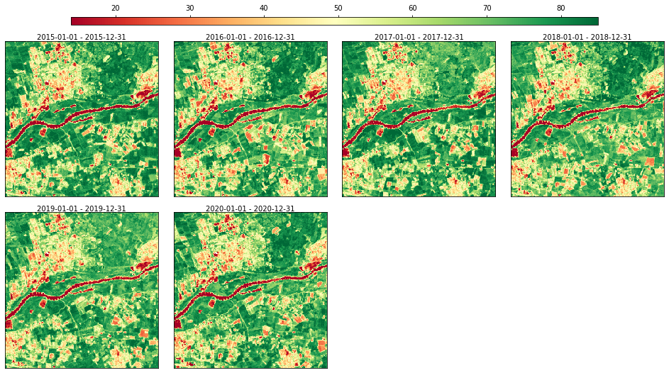
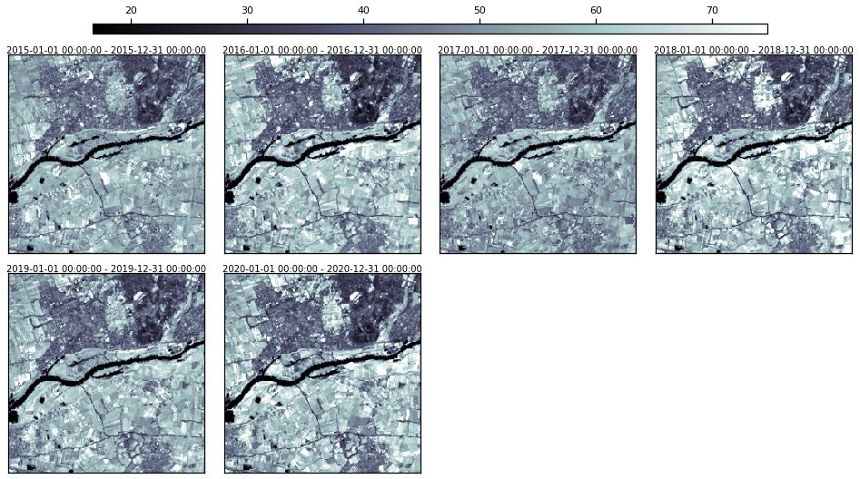
Let’s visualize the result of the annual aggregation (percentile 50th):
[12]:
rdata.plot(groups=["ndvi.yearly.p50"], cmap="RdYlGn", img_title_text="date")
[12]:
1.1. Layer groups#
RasterData supports different set of layer, organizing them by groups. Multiple bands of a raster time-series, a for example NDVI and SWIR-1 band, can be organized different groups. However it’s also possible to have different time-series size in each group, and even static raster layers without a specific date interval.
To demonstrate that let’s load another toy dataset which provides multi group support.
[13]:
import seaborn as sns
from skmap.data import toy
sns.set_context("notebook")
rdata = toy.rdata()
rdata.info["group"].value_counts().plot(kind="barh")
[08:18:18] RasterData with 50 rasters (band: 1) and 3 group(s)
[08:18:18] Reading 50 raster file(s) using 4 workers
[08:18:18] Read array shape: (256, 256, 50)
[13]:
<Axes: ylabel='group'>
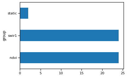
How the static group looks like?
[14]:
rdata.filter("group == 'static'").info
[14]:
| group | input_path | input_band | start_date | end_date | temporal | name | |
|---|---|---|---|---|---|---|---|
| 24 | static | /home/opengeohub/src/scikit-map/skmap/data/toy... | 1 | None | None | False | elev.lowestmode_gedi.eml_mf_30m_s_20000101_201... |
| 25 | static | /home/opengeohub/src/scikit-map/skmap/data/toy... | 1 | None | None | False | slope.percent_gedi.eml_m_30m_s_20000101_201812... |
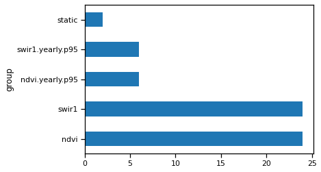
In a multi group RasterData, most of the processing tasks are executed for each group separately.
To demonstrate it, let’s run the annual aggregation by percentile 95th.
[15]:
from skmap.io import process
rdata = rdata.run(
process.TimeAggregate(time=[process.TimeEnum.YEARLY], operations=["p95"])
)
[08:18:23] Running TimeAggregate on (256, 256, 24) for ndvi group
[08:18:23] Execution time for TimeAggregate: 0.08 segs
[08:18:23] Skipping TimeAggregate for static group
[08:18:23] Running TimeAggregate on (256, 256, 24) for swir1 group
[08:18:23] Execution time for TimeAggregate: 0.07 segs
And you can see two more groups in rdata.
[16]:
rdata.info["group"].value_counts().plot(kind="barh")
[16]:
<Axes: ylabel='group'>
Let’s visualize one of them.
[17]:
rdata.plot(groups=["swir1.yearly.p95"], cmap="bone", img_title_text="date")
[17]:
2. STAC Integration#
It’s possible to connect RasterData with SpatioTemporal Asset Catalog (STAC), reading all the results from search query.
Let’s test it accessing Sentinel-2 Level-2A images through Microsoft Planetary Computing. To able run the follow code you need to have the libraries:
leafmap: Interactive maps for Jupyter notebook,
pystac-client: client built upon pystac providing higher-level functionality and ability to leverage STAC API search endpoints,
planetary-computer: client for interacting with the Microsoft Planetary Computer.
The first step is selecting a region of interest (ROI) in any where in the World. For example purposed, try to limit ROI area to 400 ha, otherwise might take to much time (> 2 min.) to download all necessary data. For larger areas consider using a cloud server co-located in West Europe or Microsoft Planetary Computing Hub.
[ ]:
import leafmap
from ipyleaflet import DrawControl, LayersControl
m = leafmap.Map(draw_control=False, measure_control=False, fullscreen_control=False)
m.add_basemap("HYBRID")
draw_control = DrawControl()
draw_control.rectangle = {
"shapeOptions": {"color": "#ff0000", "fillOpacity": 0, "opacity": 1}
}
m.add_control(draw_control)
m.add_control(LayersControl())
m
Let’s extract the bounds from the map
[19]:
from shapely.geometry import shape
geometry = shape(draw_control.data[-1]["geometry"])
bounds = geometry.bounds
print("Bounds: ", bounds[0], bounds[1], bounds[2], bounds[3])
Bounds: 5.67667 51.9616 5.710831 51.978785
and query how much Sentinel-2-l2a images are available for the ROI for specific time window through STAC.
[20]:
import os # Only necessary for opengeohub/pygeo-ide containers
os.environ["PROJ_LIB"] = "/opt/conda/share/proj/"
import planetary_computer
from pystac_client import Client
from skmap.io import RasterData
client = Client.open(
"https://planetarycomputer.microsoft.com/api/stac/v1",
modifier=planetary_computer.sign_inplace,
)
query = client.search(
max_items=1000,
collections=["sentinel-2-l2a"],
bbox=bounds,
datetime=["2023-01-01T00:00:00Z", "2023-03-30T00:00:00Z"],
)
stac_items = list(query.item_collection())
print(f"Number of STAC items: {len(stac_items):d}")
Number of STAC items: 35
The RasterData is able to read all the images from the catalog considering specific set of bands. The reading will occur only for the ROI bounds / extent.
[28]:
## See Global configuration options
## https://gdal.org/user/configoptions.html#global-configuration-options
gdal_opts = {
"GDAL_HTTP_MULTIRANGE": "YES",
"GDAL_HTTP_MERGE_CONSECUTIVE_RANGES": "YES",
"GDAL_DISABLE_READDIR_ON_OPEN": "EMPTY_DIR",
"VSI_CACHE": "FALSE",
"CPL_VSIL_CURL_ALLOWED_EXTENSIONS": ".tif",
"GDAL_HTTP_CONNECTTIMEOUT": "320",
"CPL_VSIL_CURL_USE_HEAD": "NO",
"GDAL_HTTP_TIMEOUT": "320",
"CPL_CURL_GZIP": "NO",
}
bands = ["B02", "B03", "B04", "B08", "SCL"]
rdata = RasterData.from_stac_items(stac_items, bands, verbose=True).read(
bounds=bounds, gdal_opts=gdal_opts
)
[08:22:26] RasterData with 175 rasters (band: 1) and 5 group(s)
[08:22:26] Reading 175 raster file(s) using 4 workers
[08:22:26] Transform (5.67667, 51.9616, 5.710831, 51.978785) into Window(col_off=10618.03314566466, row_off=3103.2150360064115, width=292, height=147)
[08:24:57] Read array shape: (147, 292, 175)
Let’s visualize a false color composite.
[29]:
rdata.plot(groups=["B04", "B03", "B02"], img_title_text="date", layout_col=4)
[29]:
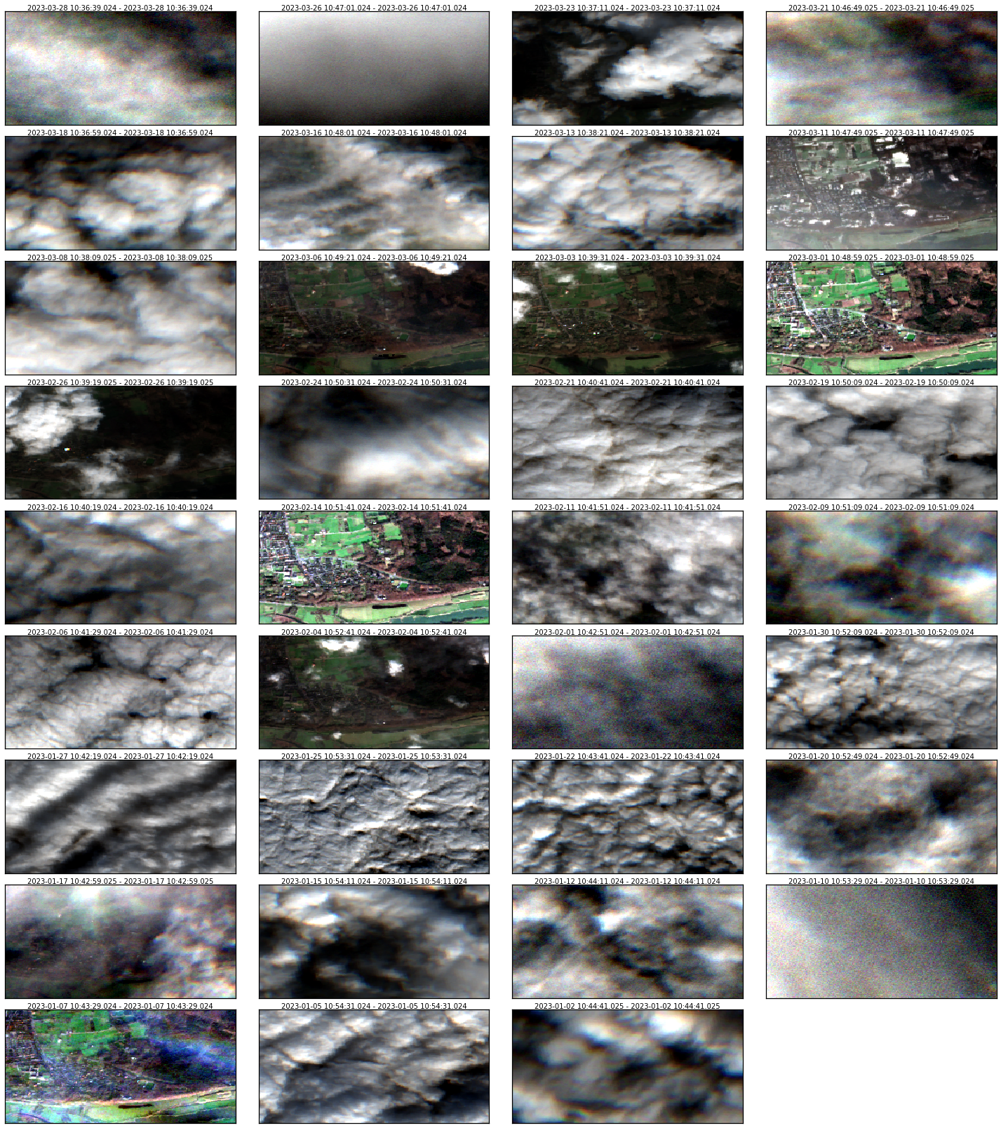
Several pixels are completely covered by clouds. It’s possible remove them using process.Calc and the Scene Classification Layer (SCL), which has the follow flag values:

This class also support the calculation several spectral indices based on expressions (NDVI, EVI2, etc). As last step, let’s run monthly aggregation by multiple time reducers.
[30]:
from skmap.io import process
rdata = (
rdata.run(
process.Calc( #
expressions={"NDVI": "((B08 - B04) / (B08 + B04))*10000"},
mask_group="SCL",
mask_values=[0, 1, 2, 3, 8, 9],
)
)
.drop(
["SCL"] # Removing SCL group
)
.run(
process.TimeAggregate(
time=[process.TimeEnum.MONTHLY], operations=["p50", "p95"], verbose=True
),
drop_input=True,
)
)
[08:25:02] Running Calc on (147, 292, 175)
[08:25:03] Execution time for Calc: 0.71 segs
[08:25:03] Dropping data and info for groups: ['SCL']
[08:25:03] Running TimeAggregate on (147, 292, 35) for B02 group
[08:25:03] Computing 3 time aggregates from 2023 to 2023
[08:25:03] Dropping data and info for B02 group
[08:25:03] Execution time for TimeAggregate: 0.08 segs
[08:25:03] Running TimeAggregate on (147, 292, 35) for B03 group
[08:25:03] Computing 3 time aggregates from 2023 to 2023
[08:25:03] Dropping data and info for B03 group
[08:25:03] Execution time for TimeAggregate: 0.08 segs
[08:25:03] Running TimeAggregate on (147, 292, 35) for B04 group
[08:25:03] Computing 3 time aggregates from 2023 to 2023
[08:25:03] Dropping data and info for B04 group
[08:25:03] Execution time for TimeAggregate: 0.08 segs
[08:25:03] Running TimeAggregate on (147, 292, 35) for B08 group
[08:25:03] Computing 3 time aggregates from 2023 to 2023
[08:25:03] Dropping data and info for B08 group
[08:25:03] Execution time for TimeAggregate: 0.08 segs
[08:25:03] Running TimeAggregate on (147, 292, 35) for NDVI group
[08:25:04] Computing 3 time aggregates from 2023 to 2023
[08:25:04] Dropping data and info for NDVI group
[08:25:04] Execution time for TimeAggregate: 0.07 segs
Here is the result:
[31]:
rdata.plot(
groups=["B04.p50", "B03.p50", "B02.p50"], img_title_text="date", layout_col=4
)
[31]:
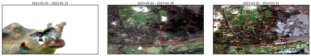
Looks good, however there are gaps in January due the lack of clear sky images. To solve this issue, let’s run the temporal gapfilling (process.SeasConvFill).
[32]:
rdata = rdata.run(process.SeasConvFill(season_size=12, return_qa=True), drop_input=True)
[08:25:04] Running SeasConvFill on (147, 292, 3) for B02.p50 group
[08:25:04] Dropping data and info for B02.p50 group
[08:25:04] Execution time for SeasConvFill: 0.02 segs
[08:25:04] Running SeasConvFill on (147, 292, 3) for B02.p95 group
[08:25:04] Dropping data and info for B02.p95 group
[08:25:04] Execution time for SeasConvFill: 0.02 segs
[08:25:04] Running SeasConvFill on (147, 292, 3) for B03.p50 group
[08:25:04] Dropping data and info for B03.p50 group
[08:25:04] Execution time for SeasConvFill: 0.02 segs
[08:25:04] Running SeasConvFill on (147, 292, 3) for B03.p95 group
[08:25:04] Dropping data and info for B03.p95 group
[08:25:04] Execution time for SeasConvFill: 0.02 segs
[08:25:04] Running SeasConvFill on (147, 292, 3) for B04.p50 group
[08:25:04] Dropping data and info for B04.p50 group
[08:25:04] Execution time for SeasConvFill: 0.02 segs
[08:25:04] Running SeasConvFill on (147, 292, 3) for B04.p95 group
[08:25:04] Dropping data and info for B04.p95 group
[08:25:04] Execution time for SeasConvFill: 0.02 segs
[08:25:04] Running SeasConvFill on (147, 292, 3) for B08.p50 group
[08:25:04] Dropping data and info for B08.p50 group
[08:25:04] Execution time for SeasConvFill: 0.02 segs
[08:25:04] Running SeasConvFill on (147, 292, 3) for B08.p95 group
[08:25:04] Dropping data and info for B08.p95 group
[08:25:04] Execution time for SeasConvFill: 0.02 segs
[08:25:04] Running SeasConvFill on (147, 292, 3) for NDVI.p50 group
[08:25:04] Dropping data and info for NDVI.p50 group
[08:25:04] Execution time for SeasConvFill: 0.02 segs
[08:25:04] Running SeasConvFill on (147, 292, 3) for NDVI.p95 group
[08:25:04] Dropping data and info for NDVI.p95 group
[08:25:04] Execution time for SeasConvFill: 0.02 segs
Here is the result:
[33]:
rdata.plot(
groups=["B04.p50.seasconv", "B03.p50.seasconv", "B02.p50.seasconv"],
img_title_text="date",
layout_col=4,
)
[33]:
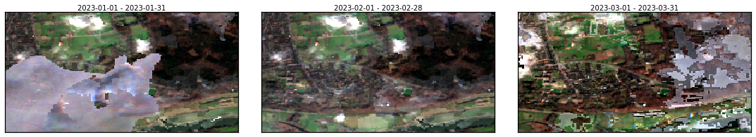
We are ready to export our data cube to folder
[34]:
rdata.to_dir("./skmap-s2-data-cube")
[08:25:05] Saving rasters in skmap-s2-data-cube
[08:25:05] Transform (5.67667, 51.9616, 5.710831, 51.978785) into Window(col_off=10618.03314566466, row_off=3103.2150360064115, width=292, height=147)
[08:25:05] Saving 60 raster files using 4 workers
[34]:
<skmap.io.base.RasterData at 0x7fa3c545b5b0>